Chapter 4 Simulations

The point of this section is to show that integrating out the mixing distributions \(V_i\) of the latent field \(\mathbf{x}\) in the variance-mean mixture representation of (2.3) leads to a significant improvement in the computational efficiency of the HMC algorithm. More speed up is obtained when leveraging on sparse matrix computations and within-chain parallelization. We simulate data from a hierarchical model where the latent field follows a RW1 process with dimension \(N \in \{2000,4000\}\). The only parameter to be estimated is the kurtosis parameter \(\eta\). We fit the model using the implementations:

Variance-Mean Mixture: 1200 iterations and 1 chain
nig_model: 1200 iterations and 1 chain
nig_model_2: 1200 iterations and 1 chain with 4 threads per chain and utilizing sparse matrix computations

The results are summarized in the following table where ESS is the effective sample size per second for the parameter \(\eta\).

Model	Total time (s)	ESS (Bulk)	ESS (Tail)
N=2000 Variance-Mean Mixture	266	0.10	0.10
N=2000 model_nig	278	1.41	2.11
N=2000 model_nig_2	77	5.30	9.56
N=4000 Variance-Mean Mixture	1132	0.01	0.04
N=4000 model_nig	884	0.32	0.54
N=4000 model_nig_2	113	2.25	4.79

Below we show the code.

4.1 Libraries and simulated data

library(ggplot2)          
library(reshape2)
library(Matrix)
library(cmdstanr)          # CmdStan R interface
library(SuppDists)         # Evaluate the density of a InvGauss distribution
source("files/utils.R")    # Several utility functions

options(mc.cores = parallel::detectCores())

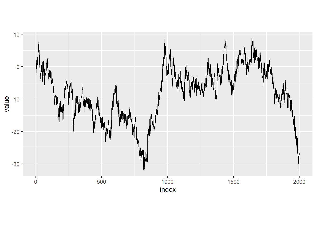
We simulate data from the following model: \(\mathbf{y}=\text{N}(\mathbf{x}, 0.7^2\mathbf{I})\), where \(\mathbf{D}_{AR1}\mathbf{x}= \mathbf{\Lambda}\).

n      <- 2000  #number of data points
m      <- 1     #rank deficiency of D
sigmay <- 0.7   #scale of the response
eta    <- 1     #leptokurtosis parameter

set.seed(123)
V   <- rinvGauss(n,nu=1,lambda = 1/eta)  #Mixing variables
L   <- rnorm(n,0,sqrt(V))                #driving noise
path <- cumsum(L) + rnorm(n, 0, sigmay)  #RW1 sample path + iid Gaussian noise

df <- data.frame(index = 1:n, path)

df_melt = melt(df, id.vars = 'index')
ggplot(df_melt, aes(x = index, y = value)) + 
    geom_line(size=0.5) + 
    theme(aspect.ratio = 0.5)

4.2 Fit with Variance-mean mixture representation

We start by fitting the model with the variance-mean mixture representation.

D    <- RW1.matrix(n)
dat1 <- list(N  = n-m,
             Ny = n,
             y  = path,
             h  = rep(1,n-m),
             meanx = 1,
             D     = as.matrix(D),
             sigmay = sigmay,
             thetaetas = 10,
             thetamus = 5)

model_stan1 <- cmdstan_model('files/stan/simulations/NIGcond.stan')

fit1 <- model_stan1$sample(data = dat1, chains = 1, iter_warmup = 200, iter_sampling = 1000)
fit1$save_object('files/stan/simulations/fit1.rds')

fit11 <- readRDS("files/stan/simulations/fit1.rds")
knitr::kable(fit11$summary(c("etas")), "simple", row.names = NA, digits=2)

variable	mean	median	sd	mad	q5	q95	rhat	ess_bulk	ess_tail
etas	0.94	0.94	0.22	0.22	0.55	1.32	1.04	27.6	27.78

4.3 Fit with nig_model

We now fit the same model with nig_model.

model_stan2 <- cmdstan_model('files/stan/simulations/modelNIG.stan')

fit2 <- model_stan2$sample(data = dat1, chains = 1, iter_warmup = 200, iter_sampling = 1000)
fit2$save_object('files/stan/simulations/fit2.rds')

fit2 <- readRDS("files/stan/simulations/fit2.rds")
knitr::kable(fit2$summary("etas"), "simple", row.names = NA, digits=2)

variable	mean	median	sd	mad	q5	q95	rhat	ess_bulk	ess_tail
etas	0.93	0.92	0.23	0.23	0.58	1.33	1	394.17	588.32

4.4 Fit with nig_model_2

We now fit the same model with nig_model_2, where we use sparse matrix computations and within-chain parallelization.

model_stan3 <- cmdstan_model('files/stan/simulations/modelNIG2.stan', cpp_options = list(stan_threads = TRUE))

fit3 <- model_stan3$sample(data = dat1, chains = 1, threads_per_chain = 4, iter_warmup = 200, iter_sampling = 1000)
fit3$save_object('files/stan/simulations/fit3.rds')

fit3 <- readRDS("files/stan/simulations/fit3.rds")
knitr::kable(fit3$summary("etas"), "simple", row.names = NA, digits=2)

variable	mean	median	sd	mad	q5	q95	rhat	ess_bulk	ess_tail
etas	0.93	0.9	0.22	0.22	0.59	1.33	1	359.04	646.72

4.5 Comparizon

Here we show the effective (bulk and tail) sample size per second for the different models

fit11$time()$total
fit11$summary("etas")["ess_bulk"]/fit11$time()$total
fit11$summary("etas")["ess_tail"]/fit11$time()$total

fit2$time()$total
fit2$summary("etas")["ess_bulk"]/fit2$time()$total
fit2$summary("etas")["ess_tail"]/fit2$time()$total

fit3$time()$total
fit3$summary("etas")["ess_bulk"]/fit3$time()$total
fit3$summary("etas")["ess_tail"]/fit3$time()$total