Chapter 6 Spatial Matérn model
6.1 Introduction
A famous class of processes is spatial statistics are stationary Gaussian processes with Matérn covariance function (Matérn (1960)). Gaussian processes with this covariance function can be obtained as a solution to the SPDE equation (Lindgren, Rue, and Lindström (2011)):
\[\begin{equation}\label{eq:SPDE} (\kappa^2 - \Delta)^{\alpha/2} X(\mathbf{s}) = \sigma \mathcal{W}(\mathbf{s}), \ \ \mathbf{s} \in \mathbb{R}^d, \end{equation}\]
where \(\kappa^2\) is a spatial scale parameter, \(\Delta=\sum_i \partial^2/\partial x_i^2\) is the Laplace operator, \(\alpha\) is a smoothness parameter, and \(\mathcal{W}(\mathbf{s})\) is a Gaussian white noise process. The approximation to discrete space in Lindgren, Rue, and Lindström (2011) uses the finite element method to the stochastic weak formulation of the previous SPDE. In 2D, it begins by expressing the process \(X(\mathbf{s})\) as a sum of piecewise triangular basis functions:
\[
X(\mathbf{s}) = \sum_{i=1}^{n}w_i\psi_i(\mathbf{s})
\]
The spatial region of interest is partitioned into a set of \(n\) non-overlapping triangles creating a mesh, where each basis function \(\psi_i(\mathbf{s})\) takes the value 1 inside a given triangle and 0 outside. The weights \(w_i\) correspond to the process \(X(\mathbf{s})\) at the nodes of the mesh. The distribution of the stochastic weights \(\mathbf{w}=[w_1,\dotsc,w_n]^T\) was found by the Galerkin method and leads to the system \(\mathbf{D}_\alpha\mathbf{w}=\mathbf{Z}\), where the Gaussian noise \(Z_i\) has variance \(\sigma^2h_i\) with \(h_i=\int\psi_i(\mathbf{s})d\mathbf{s}\) being the area of the \(i\)th basis function. When \(\alpha=2\), \(\mathbf{D}_2=\kappa^{2} \mathbf{C}+\mathbf{G}\), where:
\[\mathbf{C}_{i j}=\int\psi_i(\mathbf{s})\psi_j(\mathbf{s})d\mathbf{s}, \]
\[\mathbf{G}_{i j}=\int \nabla\psi_i(\mathbf{s})\nabla\psi_j(\mathbf{s})d\mathbf{s}. \]
The mass-lumping technique is applied to approximate \(\mathbf{C}\) with the diagonal matrix \(\text{diag}(\mathbf{h})\), so that the precision \(\mathbf{Q} = \sigma^{-2}\mathbf{D}_2 \text{diag}(\mathbf{h})^{-1}\mathbf{D}_2\) is sparse.
The random field \(X(\mathbf{s})\) at locations \(\mathbf{s}_1, \mathbf{s}_2, \dotsc\), that is \(\mathbf{x}= [X(\mathbf{s}_1), X(\mathbf{s}_2), \dotsc]^T\), is then given by \(\mathbf{x}= \mathbf{A}\mathbf{w}\), where \(\mathbf{A}\) is the projector matrix with elements \(A_{ij}=\psi_i(s_j)\). For even \(\alpha>2\) we have \(\mathbf{D}_{\alpha}= \mathbf{D}_2 \mathbf{C}^{-1} \mathbf{D}_{\alpha-2}\). All of these matrices can be computed using the function inla.mesh.fem() from the \(INLA\) package.
Bolin (2014) extended the previous results to Type-G Matérn random fields by replacing the Gaussian noise process \(\mathcal{W}(\mathbf{s})\) with normal-variance mixture distributions, from which the NIG distribution is a special case. From the more flexible noise distribution we get a Matérn random field that can better model short-term variations and sharp peaks in the latent field, or “hotspots” and “coldspots”, that is, marginal events that would be considered extreme in a Gaussian model. It was shown that the stochastic weights now follow the system \(\mathbf{D}_\alpha\mathbf{w}=\mathbf{\Lambda}(\eta^\star,\zeta^\star)\), where the matrix \(\mathbf{D}_\alpha\) is the same as in the Gaussian case seen before and \(\Lambda_i\) is NIG noise with variance \(\sigma^2h_i\), and flexibility parameters \(\eta^\star\) and \(\zeta^\star\).
6.2 Implementation
We are going to implement a latent NIG driven Matérn random field to pressure data in the northwest region of North America. This dataset was previously studied in Bolin and Wallin (2020). The main point of this section is to show how to extend a Gaussian model to non-Gaussianity in Stan and discuss the potential benefits of using a non-Gaussian latent field, rather than implementing a realistic climate model. The full Stan models are in files\stan\GaussMaternSPDE.stan and files\stan\NIGMaternSPDE.stan and here we overview the main elements of the code.
We consider no covariates for the temperature data \(\mathbf{y}\) and the projector matrix \(A\) interpolates the random field that is being modeled at the mesh nodes on the measurement locations:
\[ \mathbf{y}|\mathbf{w} \sim N(\sigma\mathbf{A}\mathbf{w},\sigma_\epsilon) \\ \mathbf{D}_2\mathbf{w} = \mathbf{\Lambda}(\eta^\star,\zeta^\star), \\ \ \text{where} \ \mathbf{D}_2 = \kappa^{2} \text{diag}(\mathbf{h})+\mathbf{G} \]
We leave out the priors for now, which will be discussed later.
6.3 Libraries and data
library(readr) # Read csv files
library(INLA) # Compute discretization mesh and FEM matrices
library(leaflet) # Interactive widgets
library(leaflet.extras) # Fullscreen control for Leaflet widget
library(cmdstanr) # CmdStan R interface
library(posterior) # Process the output of cmdstanr sampling
library(bayesplot) # Pair and trace plots
library(ggplot2) # More plots
library(GIGrvg) # Evaluate the density of a GIG distribution
source("files/utils.R") # Several utility functions
options(mc.cores = parallel::detectCores())The weatherdata.csv contains the temperature where the sample mean was subtracted from the data and the coordinates where the measurements were taken.
weatherdata <- as.data.frame(read_csv("files/data/weatherdata.csv", col_names = TRUE))6.4 Discretization mesh
Next, we create the triangle mesh to cover the studied region using the inla.mesh.2d function. The input is weatherdata[,c("lon","lat")] which are the coordinates where the measurements were taken, max.edge is the maximum allowed edge for each triangle, cutoff is the minimum allowed distance between vertexes, and max.n.strict is the maximum number of nodes allowed. From the mesh object, we obtain the matrix \(\mathbf{G}\) which describes the connectivity of the mesh nodes, the vector \(\mathbf{h}\) which contains the area of the triangles, and the projector matrix \(\mathbf{A}\) which links the location of the mesh nodes to the location of the observations. The matrix \(\mathbf{C}\) is just a diagonal matrix with the constants \(h_i\).
mesh <- inla.mesh.2d(loc = weatherdata[,c("lon","lat")], max.edge = c(1.5, 2.5), cutoff = 0.3, max.n.strict = 400)
Ny <- length(weatherdata$temp) #Number of observations
N <- mesh$n #Number of nodes
fem <- inla.mesh.fem(mesh, order=2)
G <- fem$g1
h <- diag(fem$c0)
A <- inla.spde.make.A(mesh = mesh, loc = as.matrix(weatherdata[,c("lon","lat")]))6.5 Data plot
In the next Leaflet widget, we show the data and the discretization mesh. We hid the Leaflet code here since it is quite long, but you can find it in the original Rmarkdown file.
6.6 Priors
We use the default INLA prior for \(\sigma_\epsilon\). The penalized complexity priors for the scale parameter \(\sigma\) and spatial range parameter \(\kappa\) were derived in Fuglstad et al. (2019) and their log-likelihood can be defined in the model block as:
...
//prior layer---------------------------------
//prior for sigmae
sigmae ~ inv_gamma(1, 0.00005);
//prior for rho and sigmam
target += - log(kappa) - lambda1*kappa - lambda2*sigmax/kappa;
...With the PC prior approach, we get the distribution for the priors up to a scaling constant. The hyperparameters lambda1 and lambda2 are found by relating \(\sigma\) and \(\kappa\) with more interpretable parameters, namely the marginal standard deviation \(\sigma_{marg}\) and the practical correlation range \(\rho=\sqrt{8}/\kappa\) (the distance at which the correlation is approximately 0.1). Then lambda1 and lambda2 can be found by setting the probabilities \(P(\rho<\rho_0)=\alpha\) and \(P(\sigma_{marg}>\sigma_0)=\alpha\) as follows:
# P(practic.range < 0.1) = 0.01, base model range -> infty
range.U = 0.1
range.alpha = 0.01
# P(sigma > 100) = 0.1
sigma.U = 100
sigma.alpha = 0.1
lambda1 = -log(range.alpha)*range.U/sqrt(8)
lambda2 = -log(sigma.alpha)/(sigma.U*sqrt(4*pi))The priors for the parameter \(\eta^\star\) and \(\zeta^\star\) are declared next:
...
//prior layer---------------------------------
//prior for etas
theta_etas = -4*log(alphaeta)*kappa^2;
target += log(theta_etas) - theta_etas*etas;
//prior for zetas
target += - thetazetas*fabs(zetas);
...As motivated in Cabral, Bolin, and Rue (2022) we use an exponential distribution for \(\eta^\star\) with rate \(\theta_\eta = 4\log(\alpha_{\eta})\kappa^2\). The hyperparameter \(\alpha_{\eta^\star}\) is the probability of having twice as much large marginal events compared with the Gaussian case: \(P(Q(\eta,\kappa) > 2)= \alpha_{\eta^\star}\), where: \[ Q(\eta,\kappa) = \frac{P(|X_{\eta,\kappa}(\mathbf{s})|>3\sigma_{marg}(\kappa))}{P(|X_{\eta=0,\kappa}(\mathbf{s})|>3\sigma_{marg}(\kappa))} , \] We will use \(\alpha_{\eta^\star}==0.5\), and for the Laplace prior on \(\zeta^\star\) we will use the rate parameter \(\theta_\zeta = 13\).
6.7 Stan fit with a Gaussian model
Note that the Gaussian log-likelihood for \(\mathbf{w}\) where \(\mathbf{D}\mathbf{w}=\mathbf{Z}\), and \(Z_i \sim N(0,h_i)\) is given by:
\[\log\pi(\mathbf{x}) \propto\log |\mathbf{D}| - 0.5\sum_{i=1}^n [\mathbf{D}\mathbf{w}]_i^2/h_i.\]
We will be using a non-centered parameterization to improve the inference quality. To implement a non-centered parameterization we need to invert the matrix \(\mathbf{D} = \kappa^2\mathbf{C} + \mathbf{G}\) at every iteration, so we will leverage on the result: \[ \mathbf{D}^{-1} = \mathbf{C}_1\text{diag}(\kappa^2+\mathbf{v})^{-1}\mathbf{C}_2 \] where, \[ \mathbf{C}_1 = \Gamma, \ \ \ \mathbf{C}_2 = (\mathbf{C}\Gamma)^{-1} \] with \(\mathbf{\Gamma}\) and \(\mathbf{v}\) being the eigenvector matrix and eigenvalue vector of \(\mathbf{C}^{-1}\mathbf{G} = \mathbf{\Gamma}\text{diag}(\mathbf{v})\mathbf{\Gamma}^{-1}\), respectively, which only need to be computed once, before the algorithm starts.
Lastly, the representation we use is \(\mathbf{y}\sim \text{N}(\mathbf{m}_\mathbf{y},\sigma_\epsilon^2\mathbf{I})\), where the mean is \(\mathbf{m}_y=\sigma_x\mathbf{A}\mathbf{w}\), and the stochastic weights are \(\mathbf{w}=\mathbf{D}^{-1}\mathbf{\Lambda}=\mathbf{C}_1\text{diag}(\kappa^2+\mathbf{v})^{-1}\mathbf{C}_2 \mathbf{Z}\). The model statement is :
model{
transformed parameters{
vector[N] w = diag_post_multiply(C1,inv(kappa^2+v))*C2*Z; //stochastic weights
vector[Ny] my = sigmax*A*w; //mean of observations y
}
model{
real theta_etas;
//response layer---------------------------
y ~ normal(my, sigmae);
//latent field layer--------------------------
target += -0.5*sum(Z^2 ./ h); //log-density of i.i.d Gaussian vector z
}Here we compute the matrices C1 and C2:
C <- Diagonal(N,h)
e <- eigen(solve(C)%*%G)
eigenvalues <- e$values
eigenvectors <- e$vectors
C1 <- eigenvectors
C2 <- solve(C%*%eigenvectors)
v <- eigenvaluesWe finally construct the list with all the required data.
dat1 <- list(N = N,
Ny = Ny,
y = weatherdata$temp,
h = h,
A = as.matrix(A),
C1 = as.matrix(C1),
C2 = as.matrix(C2),
v = eigenvalues,
lambda1 = lambda1,
lambda2 = lambda2,
alphaeta = 0.01,
thetazetas = 13)Then we compile and fit the model.
model_stan_Gauss <- cmdstan_model('files/stan/GaussMaternSPDE2.stan')
fit_press_temp <- model_stan_Gauss$sample(data = dat1,
chains = 4,
iter_warmup = 300,
iter_sampling = 700,
refresh = 10)
fit_press_temp$save_object("files/fits/fit_press_Gauss500.rds")Let us examine the summary of the fit for a few parameters.
fit_Gauss <- readRDS("files/fits/fit_press_Gauss500.rds")
knitr::kable(head(fit_Gauss$summary(),7), "simple", row.names = NA, digits=2)| variable | mean | median | sd | mad | q5 | q95 | rhat | ess_bulk | ess_tail |
|---|---|---|---|---|---|---|---|---|---|
| lp__ | -938.96 | -938.45 | 18.22 | 17.81 | -969.40 | -910.24 | 1.01 | 550.87 | 1057.93 |
| sigmae | 66.04 | 65.57 | 6.38 | 6.31 | 56.33 | 76.93 | 1.01 | 784.43 | 1636.17 |
| sigmax | 480.79 | 477.31 | 64.89 | 63.32 | 380.54 | 588.62 | 1.00 | 741.33 | 1378.68 |
| kappa | 0.60 | 0.59 | 0.12 | 0.12 | 0.42 | 0.82 | 1.00 | 936.83 | 1478.00 |
| Lambda[1] | 0.24 | 0.24 | 1.07 | 1.10 | -1.46 | 1.97 | 1.00 | 3739.88 | 2255.28 |
| Lambda[2] | 0.31 | 0.32 | 1.04 | 1.05 | -1.39 | 1.95 | 1.00 | 3831.08 | 1984.74 |
| Lambda[3] | 0.14 | 0.13 | 1.01 | 0.98 | -1.56 | 1.86 | 1.00 | 5439.70 | 2144.62 |
All parameters had large effective sample sizes (ess_bulk and ess_ess_tail) and acceptable \(\hat{R}\) values. Next, we have the pair and trace plots for \(\sigma_\epsilon\), \(\kappa\), and \(\sigma\).
mcmc_pairs(fit_Gauss$draws(c("sigmae", "sigmax", "kappa")),
diag_fun="dens", off_diag_fun="hex")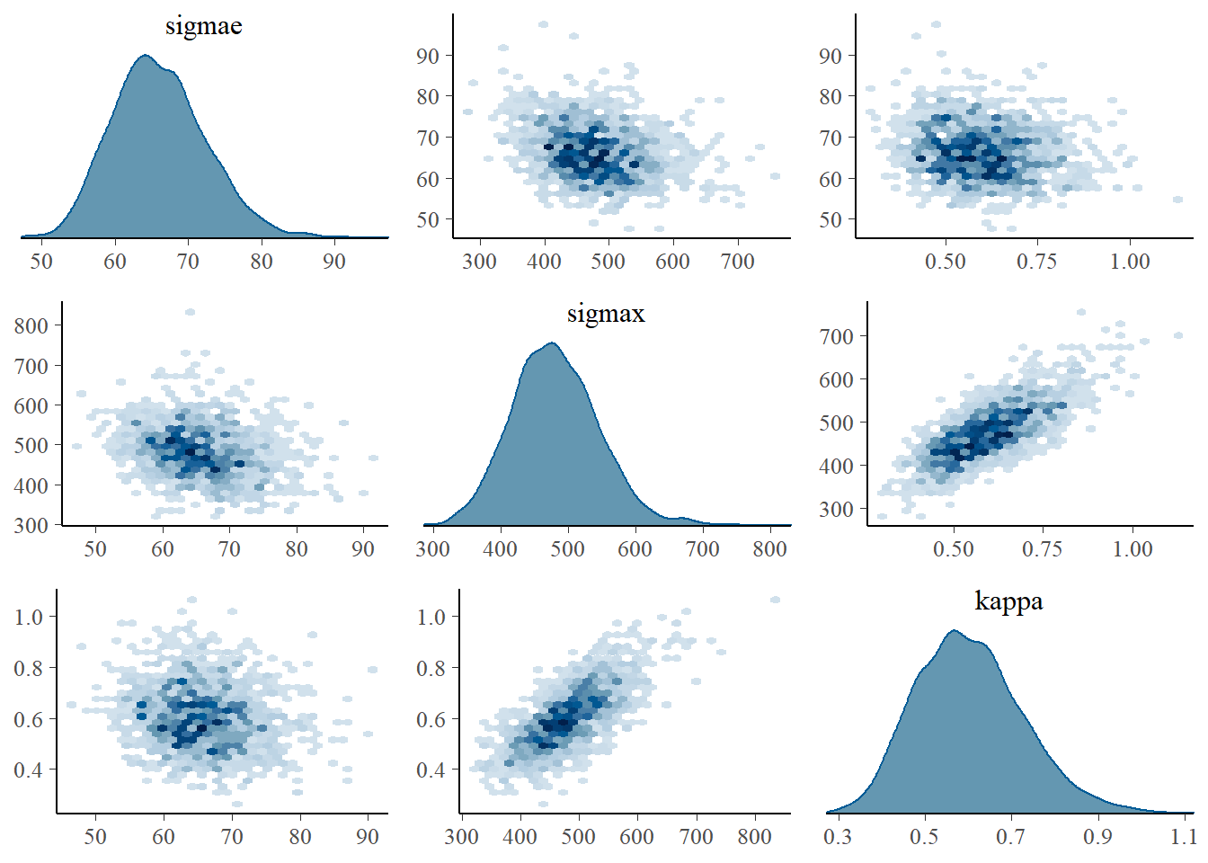
mcmc_trace(fit_Gauss$draws(c("sigmae", "sigmax", "kappa")),
facet_args = list(ncol = 2, strip.position = "left"))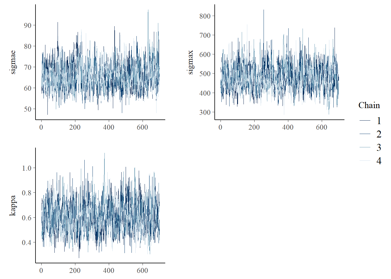
6.8 Stan fit with a NIG driving noise
The model block for the NIG model is given next. We only changed the latent field layer which is now driven by i.i.d. NIG noise.
transformed parameters{
vector[N] w = diag_post_multiply(C1,inv(kappa^2+v))*C2*Lambda; //stochastic weights
vector[Ny] my = sigmax*A*w; //mean of observations y
}
model{
real theta_etas;
//response layer---------------------------
y ~ normal(my, sigmae);
//latent field layer--------------------------
Lambda ~ nig_multi(etas, zetas, h); //nig_multi returns the density of i.i.d. nig noise
...
}We compile and fit the model next.
model_stan_NIG <- cmdstan_model('files/stan/NIGMaternSPDE2.stan')
fit_NIG_press <- model_stan_NIG$sample(data = dat1,
chains = 4,
iter_warmup = 300,
iter_sampling = 700,
refresh = 10)
fit_NIG_press$save_object("files/fits/fit_press_500.rds") The summary shows acceptable \(\hat{R}\) values and sample sizes, although compared to the Gaussian fit the effective sample sizes of \(\sigma_\epsilon\), \(\sigma\), and \(\kappa\) are lower. The posterior means of \(\sigma_\epsilon\) and \(\sigma_x\) are smaller compared with the Gaussian model which means the predictions will have a smaller variance. The posterior mean of \(\kappa\) is smaller indicating that the spatial correlation decays slower with distance. This is possibly caused by the peaks and short-term variations in the data, which are now better modeled by the latent field. The posterior distribution of \(\eta^\star\) indicates a clear departure from the Gaussian distribution, having a mean of 2.04. The 95% posterior quantiles of \(\zeta^\star\) include the 0, indicating insufficient evidence for asymmetry.
fit_NIG <- readRDS("files/fits/fit_press_500.rds")
knitr::kable(head(fit_NIG$summary(),7), "simple", row.names = NA, digits=2)| variable | mean | median | sd | mad | q5 | q95 | rhat | ess_bulk | ess_tail |
|---|---|---|---|---|---|---|---|---|---|
| lp__ | -1233.87 | -1235.16 | 29.63 | 29.41 | -1281.61 | -1184.46 | 1.01 | 264.81 | 600.53 |
| sigmae | 63.00 | 62.63 | 5.44 | 5.38 | 54.59 | 72.46 | 1.00 | 1447.13 | 1867.75 |
| sigmax | 336.77 | 332.75 | 52.60 | 53.75 | 257.84 | 427.72 | 1.00 | 520.13 | 837.36 |
| kappa | 0.37 | 0.36 | 0.08 | 0.08 | 0.25 | 0.50 | 1.01 | 473.43 | 1092.49 |
| etas | 2.04 | 1.84 | 1.07 | 0.94 | 0.70 | 4.05 | 1.02 | 234.62 | 779.20 |
| zetas | -0.01 | 0.00 | 0.06 | 0.05 | -0.11 | 0.10 | 1.00 | 2226.78 | 1852.55 |
| Lambda[1] | 0.34 | 0.22 | 1.20 | 0.89 | -1.37 | 2.43 | 1.00 | 2062.52 | 1017.63 |
mcmc_trace(fit_NIG$draws(c("sigmae", "sigmax", "kappa","etas","zetas")),
facet_args = list(ncol = 2, strip.position = "left"))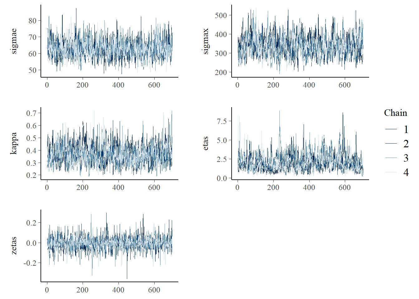
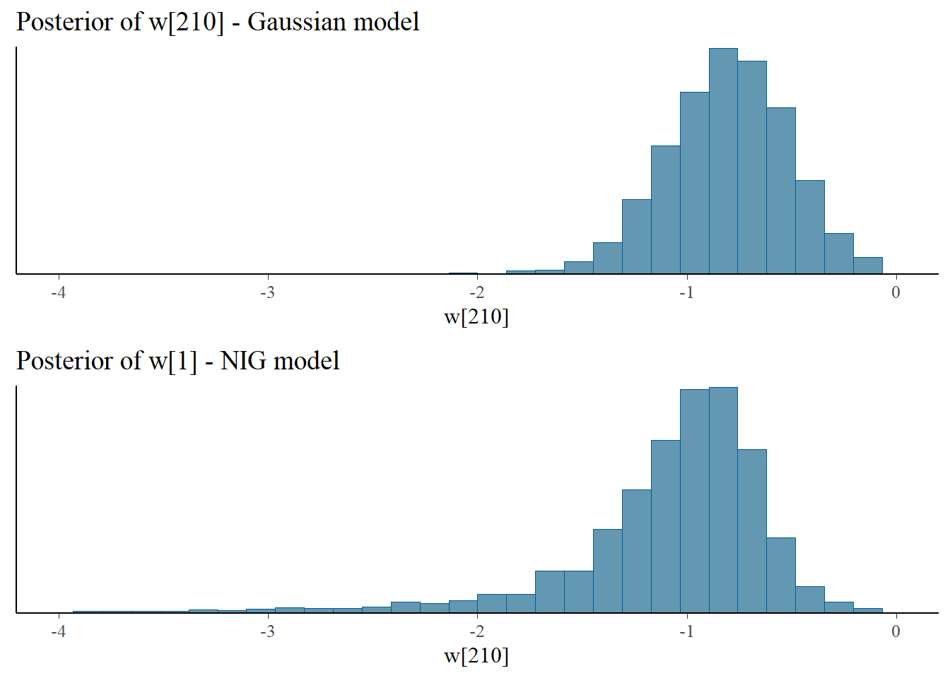
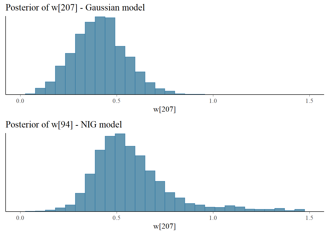
Let us look at the posterior samples of the (standardized) latent field at some nodes. We can see at nodes 210 and 207 that in the NIG model the latent field has more mass in the tails and is more skewed.
bayesplot_grid(
mcmc_hist(fit_Gauss$draws("w[210]")),
mcmc_hist(fit_NIG$draws("w[210]")),
titles = c("Posterior of w[210] - Gaussian model", "Posterior of w[1] - NIG model"),
xlim = c(-4,0)
)
bayesplot_grid(
mcmc_hist(fit_Gauss$draws("w[207]")),
mcmc_hist(fit_NIG$draws("w[207]")),
titles = c("Posterior of w[207] - Gaussian model", "Posterior of w[94] - NIG model"),
xlim = c(0,1.5)
)
6.9 Leave-one-out cross validation
We compare the Gaussian and NIG latent models using the leave-one-out cross-validation method of Vehtari, Gelman, and Gabry (2017). For these models, the elpd_loo estimates are not reliable. High Pareto-k values are often the result of model misspecification and typically correspond to data points considered outliers and surprising according to the model. We see that the NIG model has fewer observations with bad Pareto-k values.
loo_Gauss <- fit_Gauss$loo()
loo_NIG <- fit_NIG$loo()
print(loo_Gauss)##
## Computed from 2800 by 157 log-likelihood matrix
##
## Estimate SE
## elpd_loo -934.0 18.4
## p_loo 74.6 11.8
## looic 1868.0 36.7
## ------
## Monte Carlo SE of elpd_loo is NA.
##
## Pareto k diagnostic values:
## Count Pct. Min. n_eff
## (-Inf, 0.5] (good) 67 42.7% 724
## (0.5, 0.7] (ok) 48 30.6% 150
## (0.7, 1] (bad) 35 22.3% 14
## (1, Inf) (very bad) 7 4.5% 7
## See help('pareto-k-diagnostic') for details.print(loo_NIG)##
## Computed from 2800 by 157 log-likelihood matrix
##
## Estimate SE
## elpd_loo -924.0 21.4
## p_loo 71.0 14.8
## looic 1848.0 42.8
## ------
## Monte Carlo SE of elpd_loo is NA.
##
## Pareto k diagnostic values:
## Count Pct. Min. n_eff
## (-Inf, 0.5] (good) 81 51.6% 385
## (0.5, 0.7] (ok) 43 27.4% 234
## (0.7, 1] (bad) 27 17.2% 7
## (1, Inf) (very bad) 6 3.8% 1
## See help('pareto-k-diagnostic') for details.6.10 Prediction
A common problem in spatial statistics is prediction, which in our context means finding the posterior distribution of the latent field \(X(\mathbf{s})\) in locations where there are no measurement data. We will get posterior samples of \(\mathbf{x}_{pred}\) which is the latent field \(X(\mathbf{s})\) on a square grid spanning the studied region containing \(100^2\) nodes. First, we create the matrix coop containing the coordinates of the nodes in a square grid, and then inla.mesh.spde.make.A() creates the projector matrix \(\mathbf{A_p}\) that links the original mesh nodes at which we modeled the latent field to the nodes of the new square grid. Finally, \(\mathbf{x}_{pred} = \sigma \mathbf{A_p} \mathbf{w}\), where we will use the posterior samples from \(\sigma\) and \(\mathbf{w}\) obtained in Stan to generate posterior samples of \(\mathbf{x}_{pred}\).
#Square grid containing 100^2 nodes
n.grid <- 100
coop <- as.data.frame(expand.grid(seq(min(weatherdata$lon),max(weatherdata$lon),,n.grid),
seq(min(weatherdata$lat),max(weatherdata$lat),,n.grid)))
lenx <- (max(weatherdata$lon) - min(weatherdata$lon))/n.grid
leny <- (max(weatherdata$lat) - min(weatherdata$lat))/n.grid
#projector matrix for new grid
Ap <- inla.spde.make.A(mesh = mesh, loc = as.matrix(coop))
#Posterior samples from w
W_NIG <- as.matrix(as_draws_df(fit_NIG$draws("w"))[,1:N])
#Posterior samples from sigma
sigma_NIG <- as.matrix(as_draws_df(fit_NIG$draws("sigmax")))[,1]
#Posterior samples of w_pred
W_NIG_pred <- sigma_NIG * t(Ap %*% t(W_NIG)) We can visualize the posterior mean and standard deviation of \(\mathbf{x}_{pred}\) in the following Leaflet widgets, as well as the probabilities that the latent field is larger than 600 and smaller than -400 in the prediction grid. It is possible to choose between two different map providers and we choose the same color scale in the Gaussian and NIG widgets.
The posterior of the NIG latent field accurately captures the sharp peaks in the northeast region. There is a “hotpot” and “coldspot” close to one another and a Gaussian model over-smoothed these points. For instance, the largest pressure value is not covered by the 95% credible intervals of the Gaussian model, but it is covered in the NIG model. The NIG model predictions also have overall smaller standard deviations, especially in regions with few or no observations. If you hover the mouse on top of the circle markets (and deselect all projections), the observed value, posterior mean, and 95% credible intervals are shown.
6.10.0.1 NIG prediction
6.10.0.2 Gaussian prediction
6.10.1 Posterior distribution of \(\mathbf{V}\oslash\mathbf{h}\)
In the Gaussian case the vector \(\mathbf{V}\oslash\ \mathbf{h}\) is equal to \(\mathbf{1}\), and so the plot of the posterior mean of \(\mathbf{V}\oslash\ \mathbf{h}\) can be used as a diagnostic tool to assess where departures from Gaussianity occur and if a non-Gaussian model is needed at all. We prefer looking at this diagnostic plot, rather than the posterior distribution of \(\eta^\star\). The function Vposterior in ..files\utils.R can generate posterior samples of \(\mathbf{V}\oslash\ \mathbf{h}\) given posterior samples of \(\mathbf{w}\), \(\kappa\), \(\eta^\star\), and \(\zeta^\star\). We highlight the nodes where the 95% credible intervals of \(\mathbf{V}\oslash\ \mathbf{h}\) do not contain the value 1. These highlited nodes reveal the ´`tension’’ points of the Gaussian model where more flexibility is needed.
kappa <- as.matrix(as_draws_df(fit_NIG$draws("kappa")))[,1]
etas <- as.matrix(as_draws_df(fit_NIG$draws("etas")))[,1]
zetas <- as.matrix(as_draws_df(fit_NIG$draws("zetas")))[,1]
V <- Vposterior(W_NIG, kappa, G, etas, zetas, h)
Vmean <- colMeans(V) #posterior means of V/h
sel <- 1-((apply(V,2,quantile,0.05) < 1) & (apply(V,2,quantile,0.95) > 1))*1 #do 95% quantiles include the value 1?In the following widget we can visualize the posterior mean of \(\mathbf{V}\oslash\mathbf{h}\).